Take-Home-EX01

Getting Started - Geovisualisation and Analysis

Loading R packages

pacman::p_load(tmap, sf, tidyverse, knitr,dplyr,mapview,viridis)

Imorting Data

Importing geospatial data

we will import BusStop and save as sf data frame called busstop.

busstop <- st_read(dsn = "data/geospatial", layer = "BusStop")

Reading layer `BusStop' from data source 
  `D:\zzc\ISSS624\Take-home-Ex1\data\Geospatial' using driver `ESRI Shapefile'
Simple feature collection with 5161 features and 3 fields
Geometry type: POINT
Dimension:     XY
Bounding box:  xmin: 3970.122 ymin: 26482.1 xmax: 48284.56 ymax: 52983.82
Projected CRS: SVY21

Importing OD data

We will import Passenger Volumn data by using st_read()

odbus = st_read("data/Apstial/origin_destination_bus_202308.csv")

Reading layer `origin_destination_bus_202308' from data source 
  `D:\zzc\ISSS624\Take-home-Ex1\data\Apstial\origin_destination_bus_202308.csv' 
  using driver `CSV'

Warning: no simple feature geometries present: returning a data.frame or tbl_df

We will convert some data type to factor and numeric.

odbus$ORIGIN_PT_CODE <- as.factor(odbus$ORIGIN_PT_CODE)
odbus$DESTINATION_PT_CODE <- as.factor(odbus$DESTINATION_PT_CODE) 
odbus$TOTAL_TRIPS <- as.numeric(odbus$TOTAL_TRIPS)

Extracting the data

Weekday morning peak

we will extract commuting flows during the weekday morning peak

odbus6_9 <- odbus %>%
  filter(DAY_TYPE == "WEEKDAY") %>%
  filter(TIME_PER_HOUR >= 6 &
           TIME_PER_HOUR <= 9) %>%
  group_by(ORIGIN_PT_CODE,
           DESTINATION_PT_CODE) %>%
  summarise(TRIPS = sum(TOTAL_TRIPS))

`summarise()` has grouped output by 'ORIGIN_PT_CODE'. You can override using
the `.groups` argument.

Weekday afternoon peak

we will extract commuting flows during the weekday afternoon peak

odbus17_20 <- odbus %>%
  filter(DAY_TYPE == "WEEKDAY") %>%
  filter(TIME_PER_HOUR >= 17 &
           TIME_PER_HOUR <= 20) %>%
  group_by(ORIGIN_PT_CODE,
           DESTINATION_PT_CODE) %>%
  summarise(TRIPS = sum(TOTAL_TRIPS))

`summarise()` has grouped output by 'ORIGIN_PT_CODE'. You can override using
the `.groups` argument.

Weekend/holiday morning peak

we will extract commuting flows during the weekend/holiday morning peak

odbus11_14 <- odbus %>%
  filter(DAY_TYPE == "WEEKENDS/HOLIDAY") %>%
  filter(TIME_PER_HOUR >= 11 &
           TIME_PER_HOUR <= 14) %>%
  group_by(ORIGIN_PT_CODE,
           DESTINATION_PT_CODE) %>%
  summarise(TRIPS = sum(TOTAL_TRIPS))

`summarise()` has grouped output by 'ORIGIN_PT_CODE'. You can override using
the `.groups` argument.

Weekend/holiday evening peak

we will extract commuting flows during the weekend/holiday evening peak

odbus16_19 <- odbus %>%
  filter(DAY_TYPE == "WEEKENDS/HOLIDAY") %>%
  filter(TIME_PER_HOUR >= 16 &
           TIME_PER_HOUR <= 19) %>%
  group_by(ORIGIN_PT_CODE,
           DESTINATION_PT_CODE) %>%
  summarise(TRIPS = sum(TOTAL_TRIPS))

`summarise()` has grouped output by 'ORIGIN_PT_CODE'. You can override using
the `.groups` argument.

Create Hexagon grid

Use busstop to Make a hexagonal grid, set distance as 250m.

area_honeycomb_grid = st_make_grid(busstop, cellsize = 500, what = "polygons", square = FALSE)

# To sf and add grid ID
honeycomb_grid_sf = st_sf(area_honeycomb_grid) %>%
  # add grid ID
  mutate(grid_id = 1:length(lengths(area_honeycomb_grid)))

Geospatial data wrangling

Combining Busstop and Hexagon grid

Combine busstop and hexagon data set by US_STOP_N and grid_id.

busstop_hexagon <- st_intersection(busstop, honeycomb_grid_sf) %>%
  select(BUS_STOP_N, grid_id) %>%
  st_drop_geometry()

Warning: attribute variables are assumed to be spatially constant throughout
all geometries

write_rds(busstop_hexagon, "data/rds/busstop_hexagon.csv")  

Left join weekday morning peak

Now we will left join the weekday morning peak and combined hexagon grid.

od_data1 <- left_join(odbus6_9 , busstop_hexagon,
            by = c("ORIGIN_PT_CODE" = "BUS_STOP_N")) %>%
  rename(ORIGIN_BS = ORIGIN_PT_CODE,
         ORIGIN_SZ = grid_id) %>%
  group_by(ORIGIN_BS,ORIGIN_SZ) %>%
  summarise(TOT_TRIPS = sum(TRIPS))

Warning in left_join(odbus6_9, busstop_hexagon, by = c(ORIGIN_PT_CODE = "BUS_STOP_N")): Detected an unexpected many-to-many relationship between `x` and `y`.
ℹ Row 25446 of `x` matches multiple rows in `y`.
ℹ Row 3153 of `y` matches multiple rows in `x`.
ℹ If a many-to-many relationship is expected, set `relationship =
  "many-to-many"` to silence this warning.

`summarise()` has grouped output by 'ORIGIN_BS'. You can override using the
`.groups` argument.

Left join weekday afternoon peak

Now we will left join the weekday afternoon peak and combined hexagon grid.

od_data2 <- left_join(odbus17_20 , busstop_hexagon,
            by = c("ORIGIN_PT_CODE" = "BUS_STOP_N")) %>%
  rename(ORIGIN_BS = ORIGIN_PT_CODE,
         ORIGIN_SZ = grid_id) %>%
  group_by(ORIGIN_BS,ORIGIN_SZ) %>%
  summarise(TOT_TRIPS = sum(TRIPS))

Warning in left_join(odbus17_20, busstop_hexagon, by = c(ORIGIN_PT_CODE = "BUS_STOP_N")): Detected an unexpected many-to-many relationship between `x` and `y`.
ℹ Row 35040 of `x` matches multiple rows in `y`.
ℹ Row 3153 of `y` matches multiple rows in `x`.
ℹ If a many-to-many relationship is expected, set `relationship =
  "many-to-many"` to silence this warning.

`summarise()` has grouped output by 'ORIGIN_BS'. You can override using the
`.groups` argument.

Left join weekend/holiday morning peak

Now we will left join the weekend/holiday morning peak and combined hexagon grid.

od_data3 <- left_join(odbus11_14 , busstop_hexagon,
            by = c("ORIGIN_PT_CODE" = "BUS_STOP_N")) %>%
  rename(ORIGIN_BS = ORIGIN_PT_CODE,
         ORIGIN_SZ = grid_id) %>%
  group_by(ORIGIN_BS,ORIGIN_SZ) %>%
  summarise(TOT_TRIPS = sum(TRIPS))

Warning in left_join(odbus11_14, busstop_hexagon, by = c(ORIGIN_PT_CODE = "BUS_STOP_N")): Detected an unexpected many-to-many relationship between `x` and `y`.
ℹ Row 27356 of `x` matches multiple rows in `y`.
ℹ Row 3153 of `y` matches multiple rows in `x`.
ℹ If a many-to-many relationship is expected, set `relationship =
  "many-to-many"` to silence this warning.

`summarise()` has grouped output by 'ORIGIN_BS'. You can override using the
`.groups` argument.

Left join weekend/holiday evening peak

Now we will left join the weekend/holiday afternoon peak and combined hexagon grid.

od_data4 <- left_join(odbus16_19 , busstop_hexagon,
            by = c("ORIGIN_PT_CODE" = "BUS_STOP_N")) %>%
  rename(ORIGIN_BS = ORIGIN_PT_CODE,
         ORIGIN_SZ = grid_id) %>%
  group_by(ORIGIN_BS,ORIGIN_SZ) %>%
  summarise(TOT_TRIPS = sum(TRIPS))

Warning in left_join(odbus16_19, busstop_hexagon, by = c(ORIGIN_PT_CODE = "BUS_STOP_N")): Detected an unexpected many-to-many relationship between `x` and `y`.
ℹ Row 28535 of `x` matches multiple rows in `y`.
ℹ Row 3153 of `y` matches multiple rows in `x`.
ℹ If a many-to-many relationship is expected, set `relationship =
  "many-to-many"` to silence this warning.

`summarise()` has grouped output by 'ORIGIN_BS'. You can override using the
`.groups` argument.

Checking duplicate records

Check for duplicating records

duplicate1 <- od_data1 %>%
  group_by_all() %>%
  filter(n()>1) %>%
  ungroup()


duplicate2 <- od_data2 %>%
  group_by_all() %>%
  filter(n()>1) %>%
  ungroup()


duplicate3 <- od_data3 %>%
  group_by_all() %>%
  filter(n()>1) %>%
  ungroup()


duplicate4 <- od_data4 %>%
  group_by_all() %>%
  filter(n()>1) %>%
  ungroup()

Retain unique records

Use code chunk below will be used to retain the unique records.

od_data1 <- unique(od_data1)
od_data2 <- unique(od_data2)
od_data3 <- unique(od_data3)
od_data4 <- unique(od_data4)

Update od_data data frame with the grid id

Confirm if the duplicating records issue has been addressed fully.

origintrip1 <- left_join(honeycomb_grid_sf, 
                           od_data1,
                           by = c("grid_id" = "ORIGIN_SZ"))

origintrip2 <- left_join(honeycomb_grid_sf, 
                           od_data2,
                           by = c("grid_id" = "ORIGIN_SZ"))

origintrip3 <- left_join(honeycomb_grid_sf, 
                           od_data3,
                           by = c("grid_id" = "ORIGIN_SZ"))

origintrip4 <- left_join(honeycomb_grid_sf, 
                           od_data4,
                           by = c("grid_id" = "ORIGIN_SZ"))

Remove grid without value of 0

Filter out the records which TOT_TRIPS is NA.

origintrip1 = filter(origintrip1, TOT_TRIPS > 0, !(grid_id %in% c(1767, 2135)))
origintrip2 = filter(origintrip2, TOT_TRIPS > 0, !(grid_id %in% c(7068, 8361,8485,1767, 2135)))
origintrip3 = filter(origintrip3, TOT_TRIPS > 0, !(grid_id %in% c(7068, 8361,8485,1767, 2135)))
origintrip4 = filter(origintrip4, TOT_TRIPS > 0, !(grid_id %in% c(7068, 8361,8485,1767, 2135)))

Creating Interactive map

Use 4 datasets to create interactive map.

Weekday morning peak

tmap_mode("view")

tmap mode set to interactive viewing

tmap_options(check.and.fix = TRUE)
tm_shape(origintrip1)+
  tm_fill("TOT_TRIPS", 
          style = "quantile", 
          palette = "Blues",
          title = "Passenger trips") +
  tm_layout(main.title = "Passenger trips generated at planning sub-zone level",
            main.title.position = "center",
            main.title.size = 1.2,
            legend.height = 0.45, 
            legend.width = 0.35,
            frame = TRUE) +
  tm_borders(alpha = 0.5) +
  tm_scale_bar() +
  tm_grid(alpha =0.2) 

weekday afternoon peak

tmap_mode("view")

tmap mode set to interactive viewing

tmap_options(check.and.fix = TRUE)
tm_shape(origintrip2)+
  tm_fill("TOT_TRIPS", 
          style = "quantile", 
          palette = "Blues",
          title = "Passenger trips") +
  tm_layout(main.title = "Passenger trips generated at planning sub-zone level",
            main.title.position = "center",
            main.title.size = 1.2,
            legend.height = 0.45, 
            legend.width = 0.35,
            frame = TRUE) +
  tm_borders(alpha = 0.5) +
  tm_scale_bar() +
  tm_grid(alpha =0.2)

weekend/holiday morning peak

tmap_mode("view")

tmap mode set to interactive viewing

tmap_options(check.and.fix = TRUE)
tm_shape(origintrip3)+
  tm_fill("TOT_TRIPS", 
          style = "quantile", 
          palette = "Blues",
          title = "Passenger trips") +
  tm_layout(main.title = "Passenger trips generated at planning sub-zone level",
            main.title.position = "center",
            main.title.size = 1.2,
            legend.height = 0.45, 
            legend.width = 0.35,
            frame = TRUE) +
  tm_borders(alpha = 0.5) +
  tm_scale_bar() +
  tm_grid(alpha =0.2)

Weekend/holiday evening peak

tmap_mode("view")

tmap mode set to interactive viewing

tmap_options(check.and.fix = TRUE)
tm_shape(origintrip4)+
  tm_fill("TOT_TRIPS", 
          style = "quantile", 
          palette = "Blues",
          title = "Passenger trips") +
  tm_layout(main.title = "Passenger trips generated at planning sub-zone level",
            main.title.position = "center",
            main.title.size = 1.2,
            legend.height = 0.45, 
            legend.width = 0.35,
            frame = TRUE) +
  tm_borders(alpha = 0.5) +
  tm_scale_bar() +
  tm_grid(alpha =0.2)

Weekday Morning vs. Afternoon Peak

The center and southern regions of the island appear to have a higher concentration of trips during the morning peak hours, implying that more individuals commute to these locations in the morning for work or education. While the afternoon map still shows high density in these places, the distribution is more even, indicating that people are dispersing to different sections of the island, possibly returning home or heading to other sites after work or school. The distribution of hexagons in the morning peak looks to be slightly more concentrated towards the center, whereas the spread in the afternoon appears to be wider, indicating that journeys in the afternoon originate from a more diversified range of locales.

Weekend/Holiday Morning vs. Evening Peak

The morning peak looks to have a higher intensity of travels in the center area, whereas the evening peak has a more dispersed pattern, with higher trip counts in numerous periphery places. This could be due to individuals coming into the city for various morning events and then dispersing to other places in the evening. The downtown region has a distinct centralization of passenger trips. This center zone is most likely a major commercial or leisure sector that draws people even on weekends and holidays. The geographic distribution appears less concentrated on weekends/holidays than on weekdays, with more activity in outskirts and residential regions, indicating the non-work nature of travels.The nighttime map shows that there is a substantial amount of travel inside the central region, which could be attributed to dining, entertainment, and nightlife, which are common evening activities on weekends and holidays.

Getting Started - Local Indicators of Spatial Association (LISA) Analysis

loading R packages

pacman::p_load(sf, sfdep, tmap, plotly, tidyverse,zoo,Kendall)

Calculate inverse distance weight

Derive an inverse distance weights by using the code chunk below. each geometry with 8 nearest neighbors for the corresponding observation

weekday morning peak

wm_idw1 <- origintrip1 %>%
  mutate(nb = st_knn(area_honeycomb_grid,k=8),
         wts = st_inverse_distance(nb, area_honeycomb_grid,
                                   scale = 1,
                                   alpha = 1),
         .before = 1)

! Polygon provided. Using point on surface.
! Polygon provided. Using point on surface.

weekday afternoon peak

wm_idw2 <- origintrip2 %>%
  mutate(nb = st_knn(area_honeycomb_grid,k=8),
         wts = st_inverse_distance(nb, area_honeycomb_grid,
                                   scale = 1,
                                   alpha = 1),
         .before = 1)

! Polygon provided. Using point on surface.
! Polygon provided. Using point on surface.

weekend/holiday morning peak

wm_idw3 <- origintrip3 %>%
  mutate(nb = st_knn(area_honeycomb_grid,k=8),
         wts = st_inverse_distance(nb, area_honeycomb_grid,
                                   scale = 1,
                                   alpha = 1),
         .before = 1)

! Polygon provided. Using point on surface.
! Polygon provided. Using point on surface.

weekend/holiday evening peak

wm_idw4 <- origintrip4 %>%
  mutate(nb = st_knn(area_honeycomb_grid,k=8),
         wts = st_inverse_distance(nb, area_honeycomb_grid,
                                   scale = 1,
                                   alpha = 1),
         .before = 1)

! Polygon provided. Using point on surface.
! Polygon provided. Using point on surface.

Computing local Moran’s I

Compute Local Moran’s I of GDPPC at county level by using local_moran() of sfdep package.

weekday morning peak

lisa1 <- wm_idw1 %>% 
  mutate(local_moran = local_moran(
    TOT_TRIPS, nb, wts, nsim = 99),
         .before = 1) %>%
  unnest(local_moran)

weekday afternoon peak

lisa2 <- wm_idw2 %>% 
  mutate(local_moran = local_moran(
    TOT_TRIPS, nb, wts, nsim = 99),
         .before = 1) %>%
  unnest(local_moran)

weekend/holiday morning peak

lisa3 <- wm_idw3 %>% 
  mutate(local_moran = local_moran(
    TOT_TRIPS, nb, wts, nsim = 99),
         .before = 1) %>%
  unnest(local_moran)

weekend/holiday evening peak

lisa4 <- wm_idw4 %>% 
  mutate(local_moran = local_moran(
    TOT_TRIPS, nb, wts, nsim = 99),
         .before = 1) %>%
  unnest(local_moran)

Visualising local Moran’s I and p-value

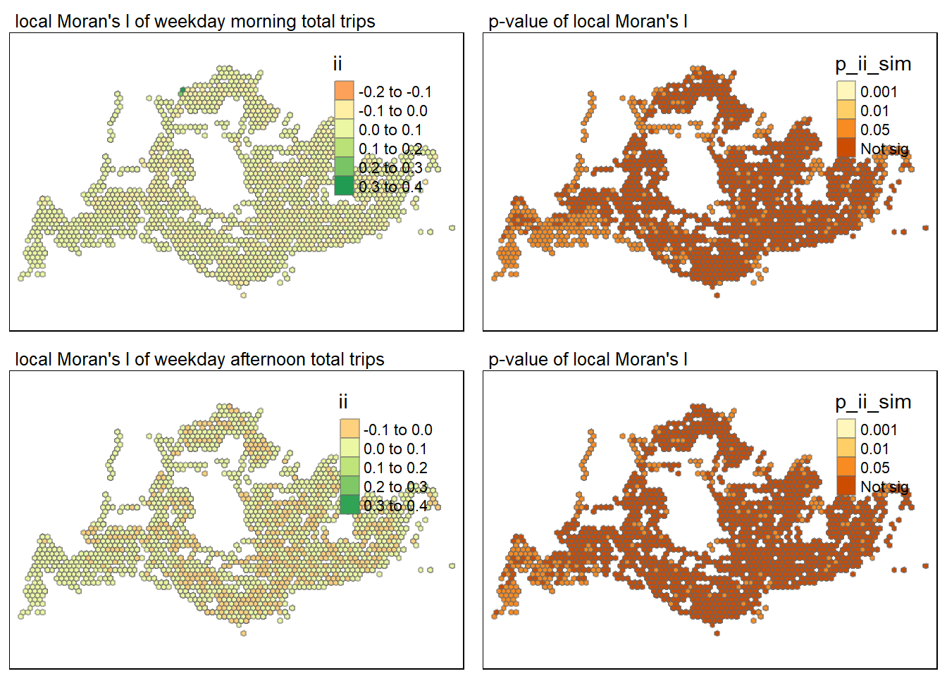
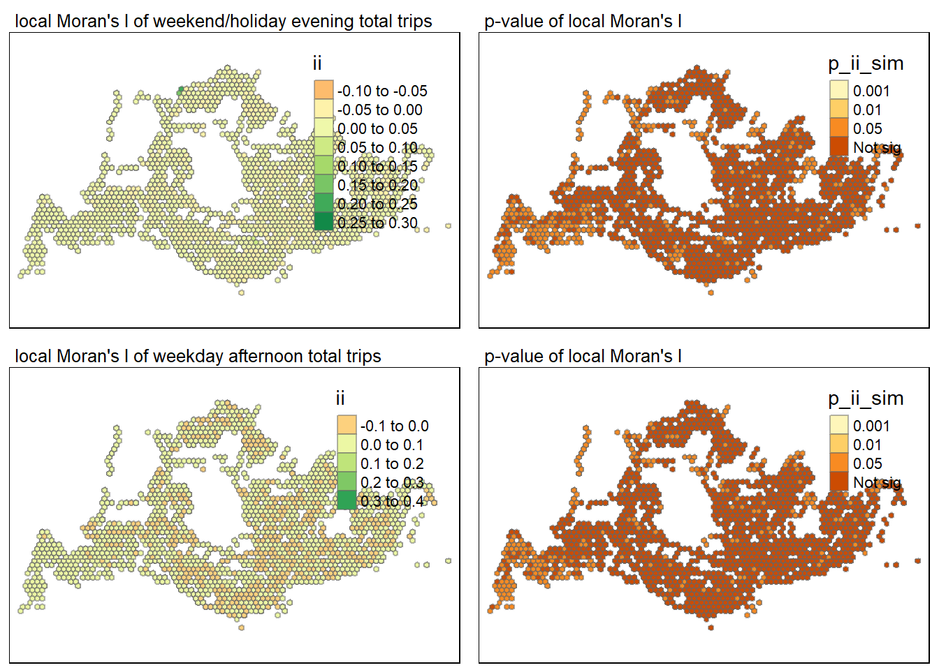
It will be better for us to plot both maps next to each other as shown below.

weekday morning and afternoon peak

tmap_mode("plot")

tmap mode set to plotting

map1 <- tm_shape(lisa1) +
  tm_fill("ii") + 
  tm_borders(alpha = 0.5) +
  tm_view(set.zoom.limits = c(6,8)) +
  tm_layout(main.title = "local Moran's I of weekday morning total trips",
            main.title.size = 0.8)

map2 <- tm_shape(lisa1) +
  tm_fill("p_ii_sim",
          breaks = c(0, 0.001, 0.01, 0.05, 1),
              labels = c("0.001", "0.01", "0.05", "Not sig")) + 
  tm_borders(alpha = 0.5) +
  tm_layout(main.title = "p-value of local Moran's I",
            main.title.size = 0.8)

#weekday afternoon peak
tmap_mode("plot")

tmap mode set to plotting

map3 <- tm_shape(lisa2) +
  tm_fill("ii") + 
  tm_borders(alpha = 0.5) +
  tm_view(set.zoom.limits = c(6,8)) +
  tm_layout(main.title = "local Moran's I of weekday afternoon total trips",
            main.title.size = 0.8)

map4 <- tm_shape(lisa2) +
  tm_fill("p_ii_sim",
          breaks = c(0, 0.001, 0.01, 0.05, 1),
              labels = c("0.001", "0.01", "0.05", "Not sig")) + 
  tm_borders(alpha = 0.5) +
  tm_layout(main.title = "p-value of local Moran's I",
            main.title.size = 0.8)

tmap_arrange(map1, map2, map3 , map4 , ncol = 2)

Variable(s) "ii" contains positive and negative values, so midpoint is set to 0. Set midpoint = NA to show the full spectrum of the color palette.

Variable(s) "ii" contains positive and negative values, so midpoint is set to 0. Set midpoint = NA to show the full spectrum of the color palette.

weekend/holiday morning and evening peak

tmap_mode("plot")

tmap mode set to plotting

map1 <- tm_shape(lisa3) +
  tm_fill("ii") + 
  tm_borders(alpha = 0.5) +
  tm_view(set.zoom.limits = c(6,8)) +
  tm_layout(main.title = "local Moran's I of weekend/holiday morning tatal trips",
            main.title.size = 0.8)

map2 <- tm_shape(lisa3) +
  tm_fill("p_ii_sim",
          breaks = c(0, 0.001, 0.01, 0.05, 1),
              labels = c("0.001", "0.01", "0.05", "Not sig")) + 
  tm_borders(alpha = 0.5) +
  tm_layout(main.title = "p-value of local Moran's I",
            main.title.size = 0.8)

#weekend/holiday  evening

tmap_mode("plot")

tmap mode set to plotting

map1 <- tm_shape(lisa4) +
  tm_fill("ii") + 
  tm_borders(alpha = 0.5) +
  tm_view(set.zoom.limits = c(6,8)) +
  tm_layout(main.title = "local Moran's I of weekend/holiday evening total trips",
            main.title.size = 0.8)

map2 <- tm_shape(lisa4) +
  tm_fill("p_ii_sim",
          breaks = c(0, 0.001, 0.01, 0.05, 1),
              labels = c("0.001", "0.01", "0.05", "Not sig")) + 
  tm_borders(alpha = 0.5) +
  tm_layout(main.title = "p-value of local Moran's I",
            main.title.size = 0.8)


tmap_arrange(map1, map2,map3,map4, ncol = 2)

Variable(s) "ii" contains positive and negative values, so midpoint is set to 0. Set midpoint = NA to show the full spectrum of the color palette.

Variable(s) "ii" contains positive and negative values, so midpoint is set to 0. Set midpoint = NA to show the full spectrum of the color palette.

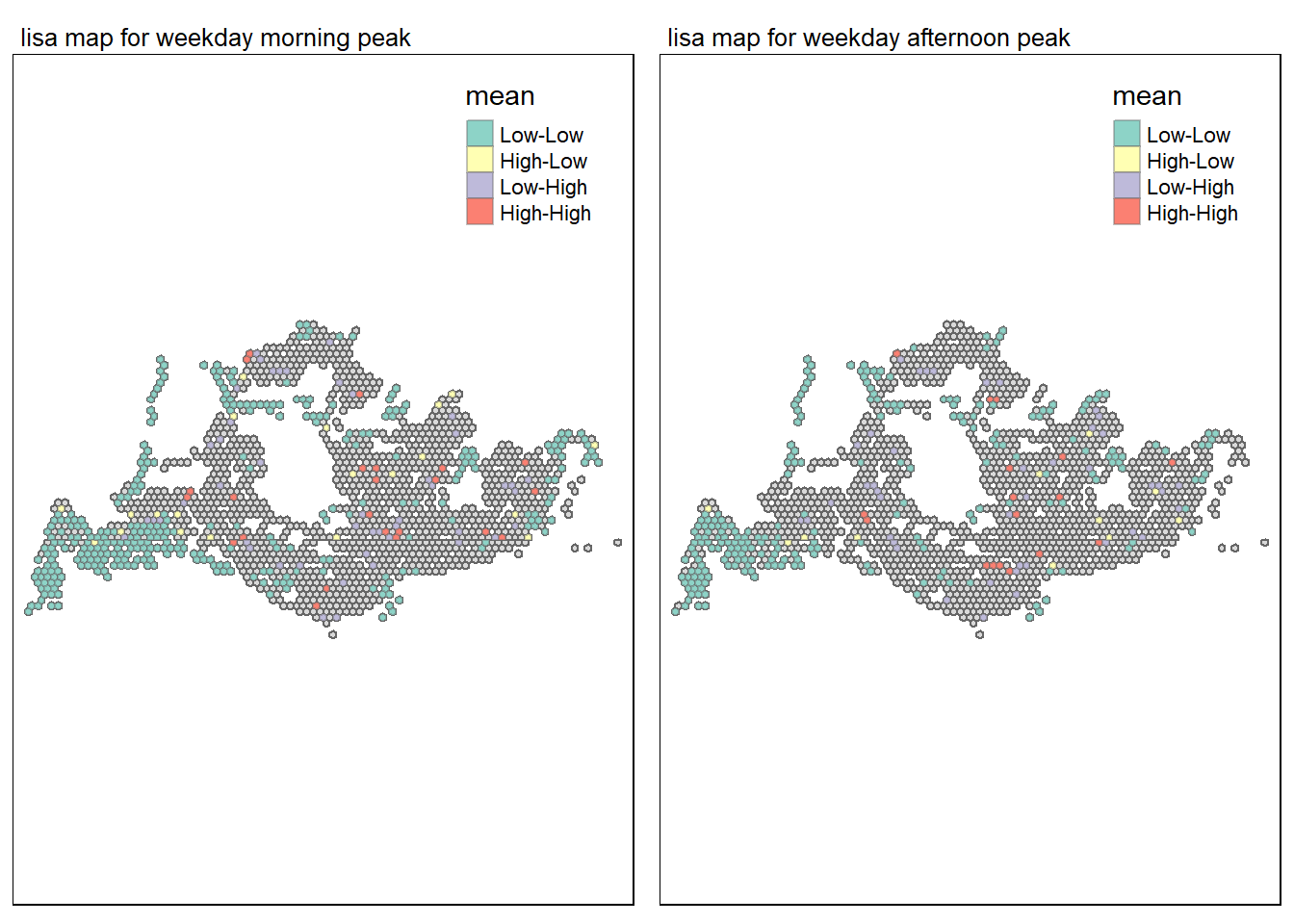
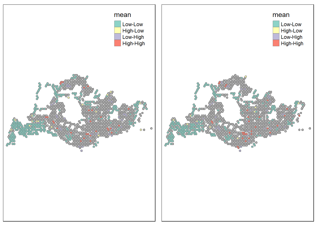
Visualising LISA map

We can find three fields contain the LISA categories. They are mean, median and pysal. In general, classification in mean will be used as shown in the code chunk below

weekday morning and afternoon peak

lisa_sig1 <- lisa1  %>%
  filter(p_ii_sim < 0.05)
tmap_mode("plot")

tmap mode set to plotting

map1 <- tm_shape(lisa1) +
  tm_polygons() +
  tm_borders(alpha = 0.5) +
tm_shape(lisa_sig1) +
  tm_fill("mean") + 
   tm_layout(main.title = "lisa map for weekday morning peak",
            main.title.size = 0.8)+
  tm_borders(alpha = 0.4)


lisa_sig2 <- lisa2  %>%
  filter(p_ii_sim < 0.05)
tmap_mode("plot")

tmap mode set to plotting

map2 <- tm_shape(lisa2) +
  tm_polygons() +
  tm_borders(alpha = 0.5) +
tm_shape(lisa_sig2) +
  tm_fill("mean") +    tm_layout(main.title = "lisa map for weekday afternoon peak",
            main.title.size = 0.8)+
  tm_borders(alpha = 0.4)

tmap_arrange(map1, map2, ncol = 2)

Warning: One tm layer group has duplicated layer types, which are omitted. To
draw multiple layers of the same type, use multiple layer groups (i.e. specify
tm_shape prior to each of them).

Warning: One tm layer group has duplicated layer types, which are omitted. To
draw multiple layers of the same type, use multiple layer groups (i.e. specify
tm_shape prior to each of them).

weekend/holiday morning and evening peak

lisa_sig3 <- lisa3  %>%
  filter(p_ii_sim < 0.05)
tmap_mode("plot")

tmap mode set to plotting

map1 <- tm_shape(lisa3) +
  tm_polygons() +
  tm_borders(alpha = 0.5) +
tm_shape(lisa_sig3) +
  tm_fill("mean") + 
  tm_borders(alpha = 0.4)

lisa_sig4 <- lisa4  %>%
  filter(p_ii_sim < 0.05)
tmap_mode("plot")

tmap mode set to plotting

map2<- tm_shape(lisa4) +
  tm_polygons() +
  tm_borders(alpha = 0.5) +
tm_shape(lisa_sig4) +
  tm_fill("mean") + 
  tm_borders(alpha = 0.4)

tmap_arrange(map1, map2, ncol = 2)

Warning: One tm layer group has duplicated layer types, which are omitted. To
draw multiple layers of the same type, use multiple layer groups (i.e. specify
tm_shape prior to each of them).

Warning: One tm layer group has duplicated layer types, which are omitted. To
draw multiple layers of the same type, use multiple layer groups (i.e. specify
tm_shape prior to each of them).

statistical conclusions

During weekday morning peak,there is a high traffic density in certain places based on high-high clustering. A few high and low outliers are also present, which would mean that some high traffic locations are close to areas with generally lower traffic.

During weekday afternoon peak:Traffic may be beginning to spread out from the high density areas in the morning, according to the decrease in high and high clustering in some area.

During weekends/holidays morning peak, Weekend morning traffic may be more equally spread than weekday traffic, as evidenced by the decrease in high and high clustering in the CBD when compared to the weekday morning peak.

During weekends/holiday evening peak:High-high clustering is more dispersed throughout the city.